
Understanding Data And its Types
Understanding Data And its Types
Everything stored in digital form is data, and it comes in two primary forms: structured and unstructured. Structured data is organized in a predefined format, often residing in relational databases or spreadsheets, where every data point fits neatly into rows and columns. For instance, a customer transaction database in a retail store—with columns for transaction ID, date, and purchase amount—epitomizes structured data that is easy to query, sort, and visualize using SQL or modern data analysis and visualization tools. In contrast, unstructured data lacks this orderly framework and encompasses diverse formats such as emails, social media posts, images, or audio recordings; consider a collection of customer reviews written in free text on a company’s website as a typical example. When it comes to storage, structured data is usually housed in relational databases that enforce strict schemas, enhancing efficiency in analysis and reporting. In contrast, unstructured data is often stored in NoSQL databases or file systems, necessitating additional processing and sophisticated algorithms to extract meaningful insights. Moreover, while structured data can be directly manipulated with standard tools and visualized with libraries like Matplotlib or Seaborn in Python, unstructured data must first be preprocessed—through techniques such as text mining or image recognition—to convert it into a structured format before any effective visualization can be created. Ultimately, structured data remains the most common source for data visualization, as even unstructured data must be organized into a structured format to facilitate clear and insightful visual analysis.
From now on, when we say Data, we mean structured data unless specifically mentioned otherwise.
What is Data?
In today’s digital world, countless buzzwords revolve around data— Big Data, Data Mining, Knowledge Discovery from Data (KDD), Data Analytics, Data Science, Machine Learning, Artificial Intelligence, Data Engineering, Business Intelligence, Data Visualization, Data Warehousing, Data Lake, and many more. At the heart of all these concepts lies one fundamental element— data itself. At its core, data is a collection of raw facts, measurements, or observations. These raw facts do not inherently carry meaning until they are processed or structured in a meaningful way.
- A single temperature reading (e.g., 30°C) is just data.
- Daily temperature readings over a month can form meaningful information about weather patterns.
- Analyzing temperature trends over decades could help generate knowledge about climate change.
Thus, data is the building block that leads to information, which further leads to knowledge and insights when analyzed appropriately.
Before we explore techniques for analyzing, processing, or visualizing data, we must first understand what data truly represents.
Data serves as the ingredient of all the above exotic techniques. Do the “ingredient” and “exotic” bring out your inner chef? Working with data requires similar finesse and discretion as a chef shows in her kitchen. I invite you to close your eyes and think of your kitchen ingredients. I know you get your favorite smell swirling in your head already. You would not cook all the ingredients in the same way. Vegetables, grains, and spices each require different preparation and storage methods. Similarly, not all data is alike. Different types of data need different techniques for preparation, analysis, storage, and, of course, visualization. For example:
- Numbers (Quantitative Data) are like raw grains, wheat, or rice—they are the staple and need structured processing.
- Text (Qualitative Data) is like spices—it adds meaning but needs interpretation.
- Dates and Time Stamps are like perishable ingredients requiring special handling.
- Categorical Labels are like recipe names—they classify things but don’t have numerical meaning.
Just as a chef must understand their ingredients before preparing a dish, a data analyst must understand the types of data before applying any analytical techniques.
With this understanding, we now move to a crucial question: What are the different types of data? We will answer this question in this chapter. The coming sections will take two broader approaches to answering this question.
- One is more statistical, where we talk about Types of Data (Continuous vs. Categorical, Ratio vs. Non-Ratio) – How data behaves mathematically.
- The second approach leans towards programming. How do programming languages treat data, and specifically, what are the “Data Types” in Python? We will understand the data from these two lenses to form one good understanding of our Data and its Types.
Understanding these distinctions is essential because the data type determines how we analyze, visualize, and interpret it. Let’s now dive into Types of Data.
Types of Data
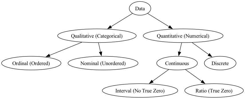
Data can be broadly categorized into Qualitative (Categorical) Data and Quantitative (Numerical) Data. Each category has further subtypes that define how the data should be interpreted and analyzed.
Qualitative (Categorical) Data
Qualitative data represents non-numeric values that describe characteristics, labels, or attributes. This type of data is classified into two categories:
Nominal Data (Unordered Categories)
- Nominal data consists of labels or names with no inherent order or ranking.
- Examples:
- Colors: Red, Blue, Green
- Gender: Male, Female, Non-binary
- Nationality: Indian, American, Canadian
- Blood Type: A, B, AB, O
Since there is no meaningful ranking or ordering, mathematical operations like addition or subtraction do not apply to nominal data.
Ordinal Data (Ordered Categories)
- Ordinal data represents categories that have a meaningful order or ranking, but the intervals between them may not be uniform.
- Examples:
- Customer Satisfaction: Poor, Fair, Good, Excellent
- Education Levels: High School, Bachelor’s, Master’s, PhD
- Military Ranks: Lieutinent, Captain, General
Even though ordinal data has an order, the differences between values are not numerically meaningful. For example, the difference between “Fair” and “Good” is not necessarily the same as the difference between “Good” and “Excellent.”
Quantitative (Numerical) Data
Quantitative data consists of numerical values that represent measurable quantities. This data type is further divided into Discrete and Continuous data.
Discrete Data
- Discrete data consists of countable values that have a finite number of possibilities.
- It typically represents whole numbers (integers).
- Examples:
- Number of students in a class: 25, 30, 40
- Number of cars in a parking lot: 50, 100, 200
- Number of pets a person owns: 0, 1, 2, 3
Since discrete data is countable, values cannot be broken down into fractions or decimals.
Continuous Data
- Continuous data represents measurable quantities that can take any value within a given range.
- It can include decimals and fractions.
- Examples:
- Height of a person: 5.6 feet, 6.2 feet
- Weight of an object: 55.3 kg, 70.8 kg
- Temperature: 36.5°C, 98.7°F
Continuous data is further divided into Interval and Ratio data.
Interval Data (No True Zero)
- Interval data has equal intervals between values, but no true zero point (zero does not mean “absence” of the quantity).
- Examples:
- Temperature in Celsius or Fahrenheit: 0°C does not mean “no temperature.”
- Calendar Years: The year 2000 is not “twice as much” as the year 1000.
- IQ Scores: A person with an IQ of 120 is not “twice as intelligent” as someone with an IQ of 60.
Since interval data lacks a true zero, ratios cannot be calculated. For example, saying “20°C is twice as hot as 10°C” is incorrect.
Ratio Data (True Zero Exists)
- Ratio data has all the properties of interval data, but also has a meaningful zero, representing the absence of the quantity.
- Examples:
- Weight: 0 kg means no weight.
- Height: 0 cm means no height.
- Speed: 0 km/h means no motion.
- Income: $0 means no income.
Since ratio data has a true zero, ratios can be meaningfully interpreted (e.g., a 100 kg object is twice as heavy as a 50 kg object).
This classification helps in selecting appropriate statistical methods and visualization techniques.
Python Data Types
Python provides a variety of built-in data types to represent different kinds of information. These types determine how data is stored in memory, how operations are carried out on the data, and how the data can be manipulated or visualized. Here’s an overview of the most commonly used Python data types:
Numeric Types
Integer (int)
- Description: Represents whole numbers (positive, negative, or zero) without any decimal component.
- Examples:
1
2
3
age = 25
count = -10
year = 2023
- Key Operations: Addition, subtraction, multiplication, integer division (
//), modulus (%), exponentiation (**).
Floating-Point Number (float)
- Description: Represents real numbers with a fractional (decimal) component.
- Examples:
1
2
3
pi = 3.14159
price = 19.99
temperature = -5.2
- Key Operations: All arithmetic operations, but results may include floating-point approximation errors.
Complex Number (complex)
- Description: Represents complex numbers in the form
a + bj, whereais the real part, andbis the imaginary part. - Examples:
1
2
z = 3 + 4j
w = -2j
- Usage: Mainly in scientific and mathematical computing (e.g., signal processing).
Boolean Type (bool)
- Description: Stores one of two values—
TrueorFalse. - Examples:
1
2
is_active = True
has_access = False
- Key Operations: Logical operations (
and,or,not), comparisons (>,<,==).
String Type (str)
- Description: Represents sequences of Unicode characters (text).
- Examples:
1
2
name = "Alice"
greeting = "Hello, World!"
- Key Operations: Concatenation (
+), slicing ([start:end]), string methods (.upper(),.lower(),.split(), etc.).
Sequence Types
Python includes multiple sequence (ordered collection) types:
List (list)
- Description: Mutable sequence of elements, can contain mixed data types.
- Example:
1
2
fruits = ["apple", "banana", "cherry"]
mixed_list = [1, "two", 3.0]
- Key Operations: Indexing, slicing, appending (
.append()), extending (.extend()), removing (.remove()), etc.
Tuple (tuple)
- Description: Immutable sequence of elements, can also contain mixed types.
- Example:
1
2
coordinates = (10.0, 20.0)
version = (3, 10)
- Key Operations: Indexing, slicing (although you cannot modify a tuple once created).
Range (range)**
- Description: Represents a sequence of integers, commonly used in loops.
- Example:
1
2
for i in range(5):
    print(i)  # 0, 1, 2, 3, 4
Set Type (set)
- Description: Unordered collection of unique elements.
- Example:
1
2
unique_numbers = {1, 2, 3}
empty_set = set()
- Key Operations: Union (
|), intersection (&), difference (-), add/remove elements.
Dictionary Type (dict)
- Description: Stores data in key-value pairs, allowing fast lookups by key.
- Example:
1
2
3
4
5
student_info = {
    "name": "Bob",
    "age": 20,
    "grades": [88, 92, 75]
}
- Key Operations: Insertion (
dict[key] = value), update, deletion, retrieving keys/values.
None Type (NoneType)
- Description: Represents the absence of a value or a null value.
- Example:
1
result = None
- Usage: Used when a variable has not been assigned a meaningful value yet.
Date and Time (via datetime module)
Although not a primitive type like int or str, Python’s standard library provides a datetime module to handle dates, times, and timestamps.
- Example:
1
2
3
import datetime
current_date = datetime.date(2025, 2, 15)
current_datetime = datetime.datetime.now()
- Key Operations: Arithmetic on dates (e.g., finding differences), comparisons, formatting (
.strftime()).
Linking Types of Data to Python Data Types
Below is a quick-reference table showing how the conceptual “Types of Data” (from statistics/data analysis) can map onto Python’s built-in data types. Note that Python doesn’t intrinsically enforce many of these distinctions; rather, context and usage determine how we treat the data.
| Statistical Data Type | Python Data Type(s) | Remarks |
|---|---|---|
| Nominal (Categorical) | str, bool, set(also object in Pandas) |
Purely labels, no inherent order. Use strings or booleans (for binary). |
| Ordinal (Categorical) | str, potentially mapped to int |
Text labels but with a meaningful sequence (e.g., "Low", "Medium", "High"). Often manually coded as integers or ordered categories. |
| Discrete (Numerical) | int |
Countable whole numbers (e.g., counts, IDs). |
| Continuous (Numerical) | float |
Measurable data with fractional values (e.g., heights, weights). |
| Interval (Continuous) | float (no strict difference in Python) |
Equal intervals but no true zero (e.g., Celsius). Contextual interpretation is important. |
| Ratio (Continuous) | float (no strict difference in Python) |
Has a true zero (e.g., weight, height). Again, context defines ratio relationships. |
| Date/Time (Ordinal/Temporal) | datetime.date, datetime.datetime |
Ordered time data. Python treats these as complex objects; arithmetic and comparison are supported. |
Important Note: Python does not enforce the statistical nuances (e.g., Interval vs. Ratio). The interpretation of whether a float is an Interval or Ratio depends on the domain context, not on Python’s internal mechanics.
Python’s built-in data types (int, float, bool, str, list, tuple, set, dict, None) lay the foundation for how data is stored and manipulated. Knowing the correct data type helps in choosing the right visualization, analysis techniques, and data structures for your project. But these are not the only data types which we will have at our disposal, when we work with data. There are Python libraries built with a focus on data analytics. We have already been introduced to two of the most popular and important libraries, NumPy (Numerical Python) and Pandas. They build upon the existing Python datatypes and provide some additional capabilities.
The below section introduces the NumPy and pandas basic data types, which are particularly crucial when using data visualization libraries in Python (e.g., Matplotlib, Seaborn, Plotly). By understanding these data types, you’ll be better equipped to organize, analyze, and visualize your data efficiently.
NumPy Data Types
NumPy is a fundamental library for scientific computing in Python. It provides a powerful n-dimensional array object, called ndarray, along with a variety of data types (dtypes) for numerical and other forms of data. The ndarray is a transformational object, which changes how we look at data, interact with it and handle complex data in Python. If you are familiar with spreadsheet programs like Excel, LibreOffice, or Google Sheets, you must have seen data in columns and rows, in tables. Handling structured data like that needs arrays.
In Pythonic terms, ndarrays are sequence type of data types. They are similar to lists, only too much faster. Also, ndarrays typically have only one type of data and thus are easier to handle and manipulate. Let us dive right into it, and see some most common types of numpy arrays that may be useful to us.
Common NumPy dtypes
- Integers
- Examples:
int32,int64 - Usage: Represent whole numbers. The suffix denotes the size of the integer in bits.
```python import numpy as np
arr_int = np.array([1, 2, 3, 4], dtype=np.int32) ```
- Examples:
- Floats
- Examples:
float32,float64 - Usage: Represent floating-point (decimal) numbers, crucial for continuous numerical computations.
1
arr_float = np.array([1.5, 2.7, 3.0], dtype=np.float64)
- Examples:
- Booleans
bool_- Usage: Store True/False values.
1
arr_bool = np.array([True, False, True], dtype=np.bool_)
- Complex
complex64,complex128- Usage: Represent complex numbers (e.g.,
1 + 2j). Useful in specialized domains like signal processing.1
arr_complex = np.array([1+2j, 3+4j], dtype=np.complex128)
- Strings & Object
str_,unicode_,object- Usage: Fixed-size or variable-size string data. Typically,
objectdtype is used for heterogeneous data types (including Python strings).1
arr_str = np.array(["apple", "banana", "cherry"], dtype=np.str_)
- Date/Time
datetime64,timedelta64- Usage: Store date-time and time-delta values, allowing vectorized operations on dates.
1
arr_date = np.array(["2023-01-01", "2023-06-15"], dtype='datetime64[D]')
Why NumPy dtypes matter for plotting
- Libraries like Matplotlib and Seaborn accept NumPy arrays as inputs.
- Ensuring the correct dtype prevents unexpected plotting behavior (e.g., trying to plot strings in a line plot).
pandas Data Types
pandas is a high-level data manipulation library built on top of NumPy. It introduces two main data structures: Series (1D) and DataFrame (2D). Each column in a DataFrame has an associated pandas dtype, which typically aligns with underlying NumPy dtypes but also includes pandas-specific types.
Common pandas dtypes
- Numeric Types
int64,float64(most common defaults)- Under the hood, these often map to NumPy’s
int64/float64.
- Boolean
bool- Similar to NumPy’s
bool_, used for storing True/False.
- Object
object- A catch-all type for text (strings) or mixed data.
1
2
3
4
5
6
7
8
9
10
import pandas as pd

df = pd.DataFrame({
    "City": ["New York", "Paris", "Tokyo"],
    "Population": [8_336_817, 2_148_327, 13_960_236]  # underscores for readability
})
print(df.dtypes)
# City          object
# Population     int64
# dtype: object
- Categorical
category- Optimized for repetitive string values or low-cardinality categories. Can also be ordered (mimicking ordinal data).
1
2
3
4
5
df["City"] = df["City"].astype("category")
print(df.dtypes)
# City          category
# Population      int64
# dtype: object
- Date and Time
datetime64[ns]- Efficiently handles dates and times for time-series analysis and plotting.
1
2
3
4
5
dates = pd.to_datetime(["2023-01-01", "2023-01-02", "2023-01-03"])
df_dates = pd.DataFrame({"Date": dates})
print(df_dates.dtypes)
# Date    datetime64[ns]
# dtype: object
- Timedelta
timedelta64[ns]- Represents time differences or durations (e.g., days between two dates).
Why pandas dtypes matter for plotting
- Many plotting libraries can take a pandas DataFrame directly.
- Using the correct dtype (e.g.,
datetime64for date columns,categoryfor categorical variables) makes plotting functions smarter about axis scales and plot types.
Example: Checking and Converting dtypes in pandas
1
2
3
4
5
6
7
8
9
10
11
12
13
14
15
16
17
18
19
20
21
22
23
24
import pandas as pd

data = {
    "Name": ["Alice", "Bob", "Charlie"],
    "Age": [25, 30, 35],
    "Registered_On": ["2023-01-01", "2022-12-15", "2023-05-10"]
}

df = pd.DataFrame(data)

# Check DataFrame dtypes
print(df.dtypes)
# Name             object
# Age              int64
# Registered_On    object
# dtype: object

# Convert 'Registered_On' to datetime
df["Registered_On"] = pd.to_datetime(df["Registered_On"])
print(df.dtypes)
# Name                     object
# Age                       int64
# Registered_On    datetime64[ns]
# dtype: object
By converting Registered_On to datetime64[ns], plotting libraries can automatically recognize this column as a date axis, enabling time-series plotting.
Linking Types of Data (Conceptual) to NumPy/pandas dtypes
Below is a reference table linking statistical/data-analysis concepts to common NumPy/pandas dtypes. Keep in mind that the interpretation (e.g., Interval vs. Ratio) isn’t enforced by the library—it’s about how you use the data.
| Conceptual Data Type | Likely NumPy dtype | Likely pandas dtype | Notes |
|---|---|---|---|
| Nominal Categorical | object (often strings) |
object or category |
E.g., city names, labels. category is efficient for repeated values. |
| Ordinal Categorical | object (manual ordering) |
category (ordered=True) |
E.g., “Beginner”, “Intermediate”, “Expert”. You can explicitly set an order. |
| Discrete Numerical | int32, int64 |
int64 |
Counts, IDs. The number of bits may vary (32, 64) depending on size. |
| Continuous Numerical | float32, float64 |
float64 |
Real-valued data (e.g., height, weight, temperature). Float precision can matter. |
| Interval (Continuous) | float32, float64 |
float64 |
Distances between values matter, no true zero (e.g., Celsius). Context is key. |
| Ratio (Continuous) | float32, float64 |
float64 |
Distances and absolute zero matter (e.g., weight, length). Context is key. |
| Date/Time (Ordinal) | datetime64[D], etc. |
datetime64[ns] |
Time-series data. Python/pandas can do time arithmetic and grouping by date. |
Key Takeaways
- NumPy:
- Offers a robust ndarray structure with various dtypes (
int,float,bool,datetime64, etc.). - Most plotting libraries accept NumPy arrays as inputs, so getting the dtype right is essential.
- Offers a robust ndarray structure with various dtypes (
- pandas:
- Builds on NumPy’s fundamentals, introducing Series and DataFrame.
- Supports categorical data (
category), datetime (datetime64[ns]), and more for optimized data handling. - Automatic plotting compatibility with libraries like Matplotlib, Seaborn, and Plotly.
- Interpretation Matters:
- Libraries don’t enforce Interval vs. Ratio or Nominal vs. Ordinal—this is a conceptual distinction.
- Choose your dtypes carefully to reflect real-world meaning.
- Practical Implications:
- Correct dtypes ensure efficient memory usage, faster operations, and smooth plotting experiences.
categoryin pandas is particularly useful for large categorical columns.datetimedtypes streamline time-series analysis and visualizations.
Armed with this overview, you can confidently choose the right NumPy and pandas dtypes for your data, ensuring effective data manipulation and high-quality visualizations.
Conclusion
In this chapter, we explored the foundational concept of what data is and why it matters, followed by a detailed look at different data classifications—nominal, ordinal, discrete, continuous, interval, and ratio. We also examined how these conceptual types map onto Python’s built-in data types, as well as NumPy and pandas data types, which play a vital role in efficient data manipulation and visualization. Understanding these distinctions sets the stage for selecting appropriate statistical methods, choosing the right charts, and generally making sense of data in a structured manner.
With this comprehensive grounding in data types, we are now ready to move forward to the next critical steps in the data pipeline: Data Cleaning and Preprocessing. The next chapter will focus on the methods and best practices for dealing with missing values, outliers, and inconsistent formats, ensuring that data is of the highest possible quality before diving into deeper analysis and visualization.